1. Visual Correspondence(1)

게시 2024/05/02

By UI-JIN KIM 11 분읽는 시간

Sparse Correspondence

특정 점들을 통해 이미지간의 매칭을 수행하는 것
즉, 이 특징점들을 추출하여 Vector화할 때, 다음 두가지 Property를 구현하는 것이 중요하다.

Robustness: 비슷한 Feature들은 가까운 거리에 존재하는 것
Distinctiveness: 다른 Feature들은 먼 거리에 존재하는 것

(Next: Dense Correspondence: flow예측과 같이 모든 점들을 활용해 Pixel간의 매칭을 수행하는 것)

1. Classical Method

Image Matching의 Classical한 Pipeline은 다음과 같다.

Feature Detect	$\rightarrow\qquad$ Feature Descriptor	$\rightarrow\qquad$ Matching
$\begin{bmatrix} \text{'Salient'}\\ \text{Repeatable'} \end{bmatrix}$한 Point 찾기	점의 특징을 수학적으로 표현	$N \times M$개의 Matching Candidate 비교

※ Salient: 두드러진
※ 8-Point Algorithm: 8개의 Matching Point를 통해 두 이미지의 기하학적 관계를 추정하는 알고리즘

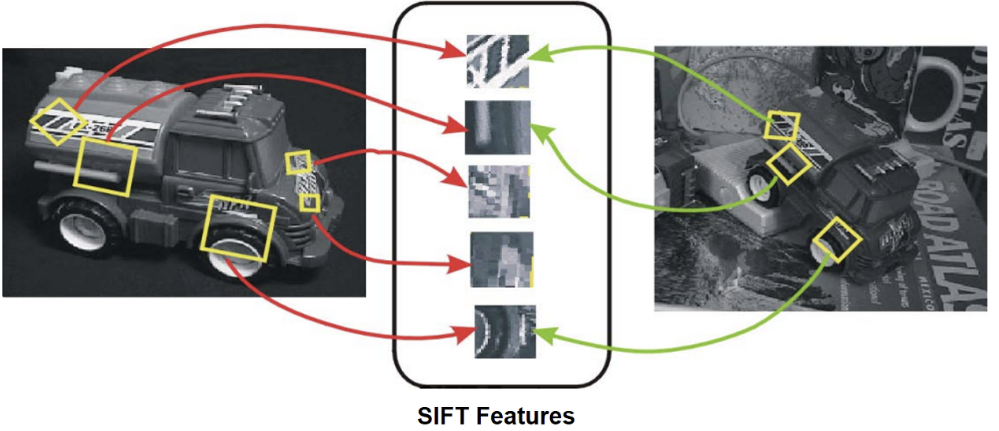
1) SIFT

Step1: Detection
SIFT는 Blobs Detector로, Feature Detect시에 Blob한 지점들을 찾는다.
(※ Harris Corner: Corner Detector)
또 추가적으로 Scale Invarient하게 동작할 수 있도록 설계한다.
Blob을 찾을 수 있는 방법에는 다음 2가지 방법이 있다.
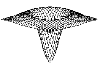
LoG(Laplacian of Gaussian) DoG(Difference of Gaussian)

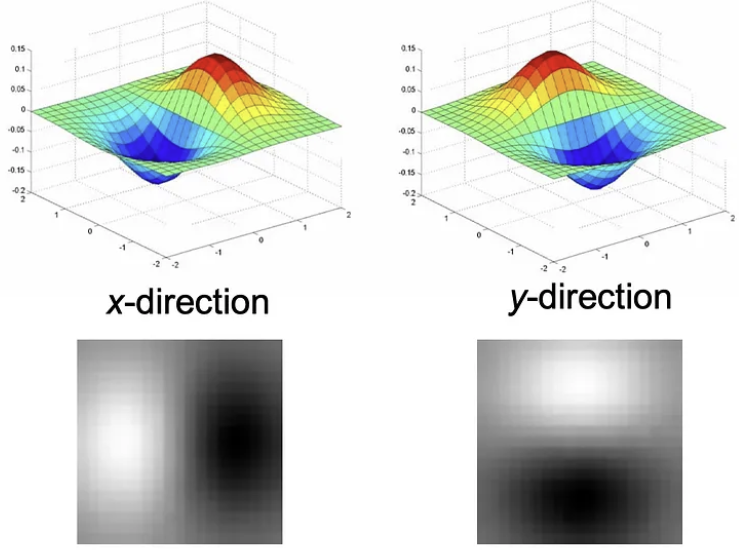
Gaussian Filter에 Laplacian을 적용한 Filter,
BandPass Filter, Blob한 점에서 큰 반응을 보임
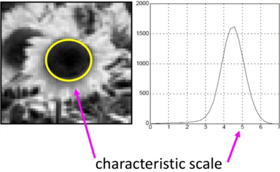
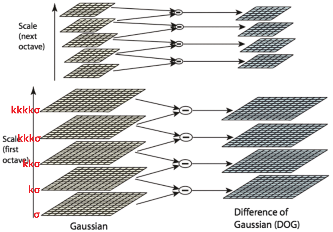
($\sigma$를 변화시키며 가장 큰 반응이 오는 값을 찾음) Gaussian Pyramid에서 같은 Octave에 있는
이미지 2개를 뺀 값으로 LoG에 근사할 수 있다.
LoG이미지나, DoG이미지들을 필터의 크기나 이미지의 크기를 조절해가며 Pyramid 구조로 쌓음으로써 Scale Invarient하게 동작하도록 설계할 수 있다.
여기서 유의해야 할 점이 LoG Pyramid를 사용할 경우 다음과 같은 문제가 발생한다는 점이다
Computational Cost가 크다
미분 시 Noise가 증폭되는데 Log는 미분을 두번한다.
즉, 위와 같은 문제들을 방지하기 위해 SIFT에서는 DoG Pyramid를 사용한다.
\[\Downarrow\]
3D NMS KeyPoint Localization
$D(\mathbf{x}) = D + \frac{\partial D^T}{\partial \mathbf{x}} \mathbf{x} + \frac{1}{2} \mathbf{x}^T \frac{\partial^2 D}{\partial \mathbf{x}^2}\mathbf{x}$
$D(\mathbf{x})’ = 0$
(DoG 이미지($D$)의 2차 근사의 극값)
$\qquad \Downarrow$

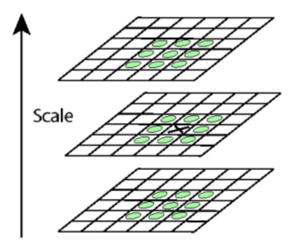
위에서 구한 DoG Scale Space에서 상하좌우
28개 점과 비교하여 가장 큰 점을
Corner후보군으로 선택한다. 3D NMS를 통해 고른 점은 Corner뿐만
아니라 Edge도 포함되어 있다.
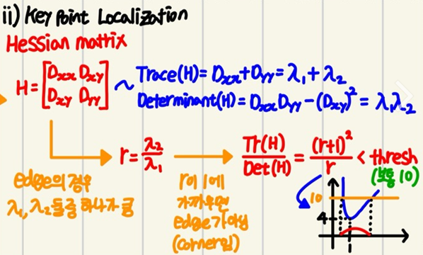
SIFT에서는 이를 걸러줄 방법으로
DoG 이미지의 Hessian Matrix를 이용한다.
\[\Downarrow\]
지금까지 ⅰ) Dog를 통해 특징점 후보군 추출, ⅱ) 3D NMS + KeyPoint Localization으로 특징점의 위치와 크기를 확정하였고
이제 ⅲ) 특징점의 방향을 할당해 줄 차례이다.
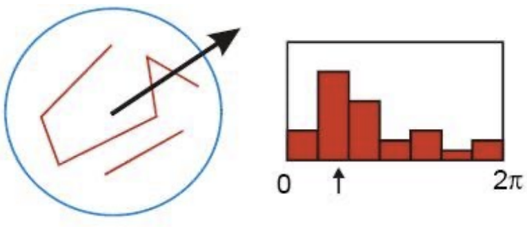
Orientation Assignment

특징점의 위치에서 Scale범위 내의 모든 점들에 대해
다수가 가리키는 방향으로 Keypoint의 방향을 설정한다.
이때, Dominant한 방향이 여러개일 경우
각각의 방향을 가지는 Blob을 여러개 설정한다.
Step2: Description
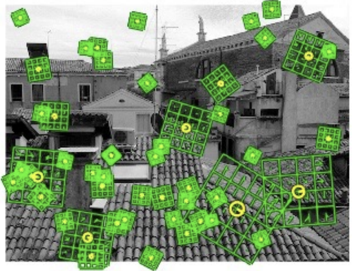
Step1에서 KeyPoint를 구했고, 이제 Matching을 위해 서로 다른 KeyPoint를 식별/구분할 수 있는 Finger Print를 만들어야 한다.
이를 Descriptor라고 한다.
Image에서 Keypoint별로 $4 \times 4$개의 Window로 나눈다.
그리고 이 Window를 다시 $4 \times 4$개의 Sub-Window에
할당한다. (총 $16 \times 16$으로 나뉨)
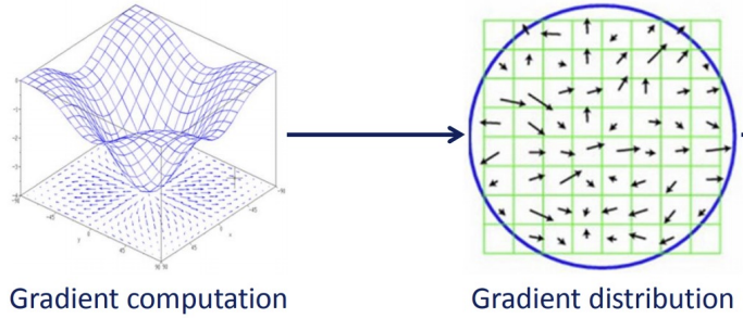
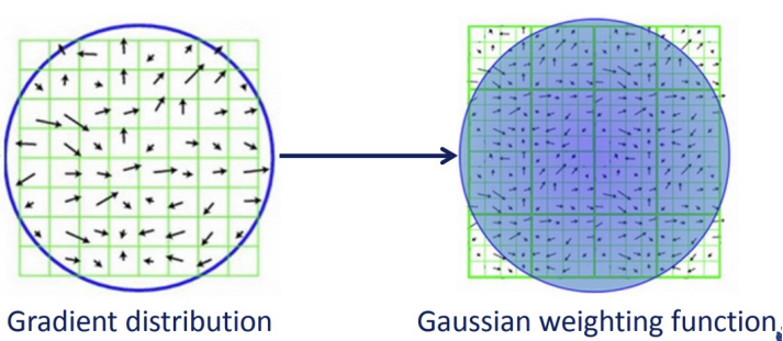
마지막으로 각 구역별로 Image Pixel값에 기반해
Gradient를 계산한다.
이 Gradient들을 Noise에 Robust하게 작동하도록
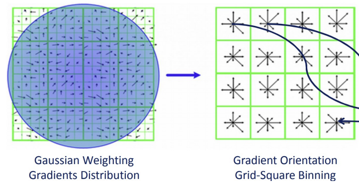
하기 위해 Gaussian Filter를 적용해준다.
이제 Window별로 할당된 모든 구역에 대해
8개의 방향을 갖는 Orientation Histogram을 그린다.
(Window당 $8 \times 4 \times 4 = 128$차원의 Vector가 생긴다.)
완성

3D NMS	KeyPoint Localization
	$D(\mathbf{x}) = D + \frac{\partial D^T}{\partial \mathbf{x}} \mathbf{x} + \frac{1}{2} \mathbf{x}^T \frac{\partial^2 D}{\partial \mathbf{x}^2}\mathbf{x}$ $D(\mathbf{x})’ = 0$ (DoG 이미지($D$)의 2차 근사의 극값) $\qquad \Downarrow$
위에서 구한 DoG Scale Space에서 상하좌우 28개 점과 비교하여 가장 큰 점을 Corner후보군으로 선택한다.	3D NMS를 통해 고른 점은 Corner뿐만 아니라 Edge도 포함되어 있다. SIFT에서는 이를 걸러줄 방법으로 DoG 이미지의 Hessian Matrix를 이용한다.

2. Deep Learning

1) Feature Descriptor(Metric Learning)

Metric Learning에서는 Hinge Loss를 주로 사용하여 Matching여부의 결정경계를 찾는다.

\[Loss(y, \hat{y}) = \min \limits_w \begin{Bmatrix} \frac{\lambda}{2} \Vert w \Vert_2 + \sum \limits_{i=1}^N \text{max}(0, 1-y_i\hat{y}) \end{Bmatrix}\]

※ Metric Learning: 입력 이미지간의 유사도(거리)를 학습하는 모델

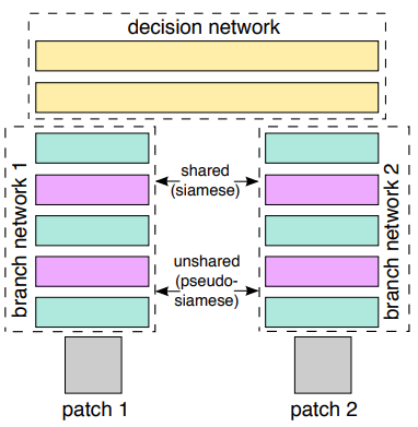
Paper1: DeepCompare
※ Network: Descriptor 역할
※ Decision Layer: Matching 역할
Architecture
2-Channel Model
2개의 Patch를 Channel방향으로 Concatenate하여 입력함

문제점
Patch Pair간의 중복된 부분을 Pair-Wise하게 계산하기 때문에
Descriptor의 재사용이 불가능하다.
(ex. [P1, P2]에서 사용한 Descriptor는 [P1, P3]에서 사용 불가 )
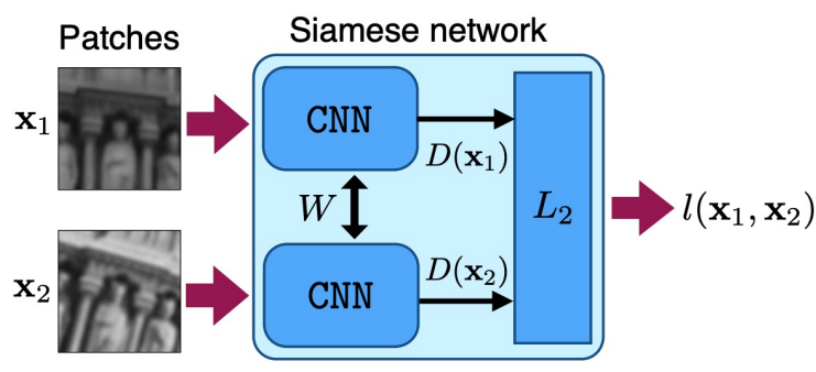
$\Rightarrow$ Computational Cost가 큼
Siamese Model
1개의 Patch($P_1$)에 대해 Descriptor를 추출하고, 이 가중치를
그대로 사용하여 다른 Patch($P_2$)의 Descriptor를 추출

$\Rightarrow$ $P_1$과 ($P_3, P_4, P_5…$)를 비교할 때,
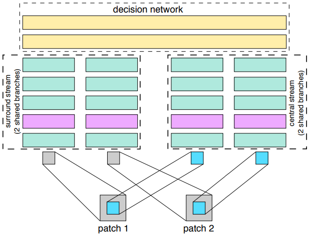
$\quad$ 추가적인 계산이 필요 없다.
2-Channel 2-Stream Model
2개의 독립적인 Stream을 통해 Patch를 비교하는 방식
(2-Channel모델 2개를 합쳐놓은 모델)

ⅰ. Stream 1: 두 Patch의 중심부를 비교하는 Stream
ⅱ. Stream 2: 두 Patch의 주변부를 비교하는 Stream

$\Rightarrow$ 다양한 Receptive Field에서 비교할 수 있음
$\Rightarrow$ Decision Network가 여전히 필요하다는 단점
Paper2: DeepDesc
Architecture
별도의 Decision Network없이 Siamese Network에서 추출한
Descriptor Vector들의 L2-Norm을 출력

Pairwise Hinge Loss
$l(\mathbf{x}_1, \mathbf{x}_2) = \begin{cases} \Vert D(\mathbf{x}_1) - D(\mathbf{x}_2) \Vert_2, \quad p_1 = p_2 \\ \text{max}(0, C-\Vert D(\mathbf{x}_1) - D(\mathbf{x}_2) \Vert_2), \quad p_1 \neq p_2\end{cases}$
Hard Negative Mining
Hard Negative란 실제로는 Negative인데 Positive라고 잘못 예측하기 쉬운 데이터를 말한다.
반면에 Easy Negative란 실제로도 Negative이고 예측도 Negative라고 예측하기 쉬운 데이터를 말한다.
주로 False Positive Sample이 Hard Negative데이터가 되는데, 이 이유는 보통 Positive에 해당하는 것을 학습하는 것을 목표로 하기 때문에 잘못 예측한 False Negative Sample은 잘 고려하지 않기 때문이다.
Hard Negative Mining은 이런 Sample들을 추출해 데이터셋에 포함시켜 학습하는 방법이다.
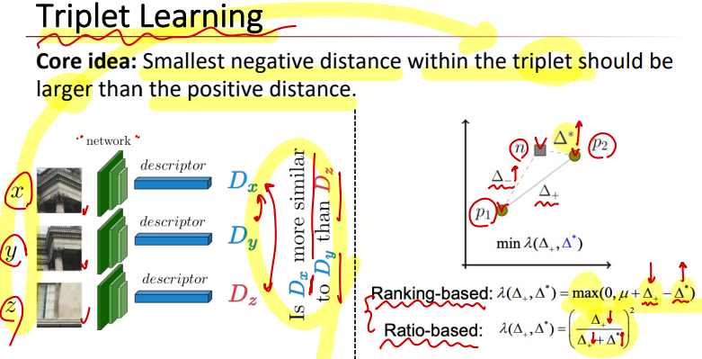
Paper3: Triplet Learning

Architecture
2-Channel Model	2개의 Patch를 Channel방향으로 Concatenate하여 입력함 문제점 Patch Pair간의 중복된 부분을 Pair-Wise하게 계산하기 때문에 Descriptor의 재사용이 불가능하다. (ex. [P1, P2]에서 사용한 Descriptor는 [P1, P3]에서 사용 불가 ) $\Rightarrow$ Computational Cost가 큼
Siamese Model	1개의 Patch($P_1$)에 대해 Descriptor를 추출하고, 이 가중치를 그대로 사용하여 다른 Patch($P_2$)의 Descriptor를 추출 $\Rightarrow$ $P_1$과 ($P_3, P_4, P_5…$)를 비교할 때, $\quad$ 추가적인 계산이 필요 없다.
2-Channel 2-Stream Model	2개의 독립적인 Stream을 통해 Patch를 비교하는 방식 (2-Channel모델 2개를 합쳐놓은 모델) ⅰ. Stream 1: 두 Patch의 중심부를 비교하는 Stream ⅱ. Stream 2: 두 Patch의 주변부를 비교하는 Stream $\Rightarrow$ 다양한 Receptive Field에서 비교할 수 있음

Architecture
	별도의 Decision Network없이 Siamese Network에서 추출한 Descriptor Vector들의 L2-Norm을 출력 Pairwise Hinge Loss \(l(\mathbf{x}_1, \mathbf{x}_2) = \begin{cases} \Vert D(\mathbf{x}_1) - D(\mathbf{x}_2) \Vert_2, \quad p_1 = p_2 \\ \text{max}(0, C-\Vert D(\mathbf{x}_1) - D(\mathbf{x}_2) \Vert_2), \quad p_1 \neq p_2\end{cases}\)

2) Orientations

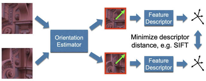
이 후에는 Orientation까지 Neural Network로 추측하는 모델도 등장하게 된다.
즉, 이 Network를 사용하여 End-To-End로 Feature Descriptor를 추출하는 모델을 완성할 수 있다.

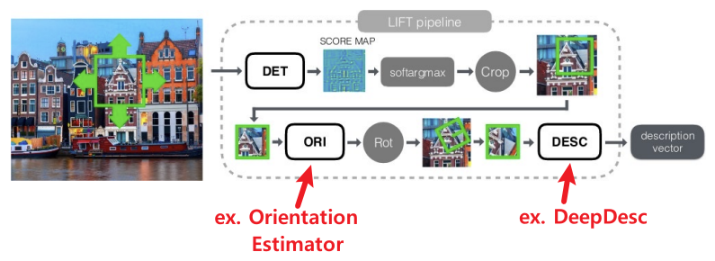
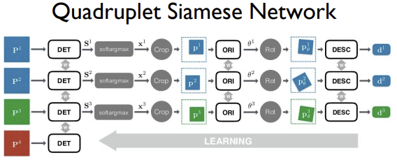
Paper1: LIFT
(아마 처음으로 End-To-End Feature Descriptor를 만든 논문인듯?)
Pipeline Quadruplet Siamese Netowrk

($\approx$ Triplet Network)
Test Time에는 Score Map을 추출하고 난 후, Score Pyramid를 만들고 NMS를 수행하는 과정을 통해 SIFT의 DoG와 비슷한 과정으로 구현하였다.
Paper2: SuperPoint
Paper3: D2Net

Pipeline	Quadruplet Siamese Netowrk
	($\approx$ Triplet Network)

3) Matching

Classical한 Matching 방법에는 다음이 있다.

NM	MNN

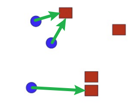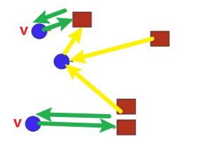Matching하고자 하는 점에서 가장 가까운 점을 찾는 것	Matching의 주체와 대상이 모두 가까운 경우에만 수행하는 것

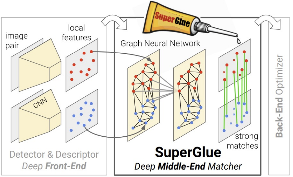
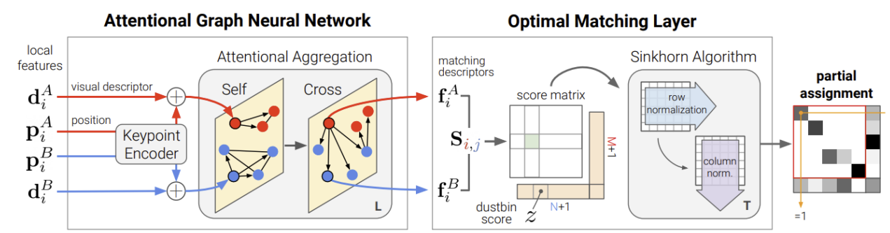
Paper1: SuperGlue
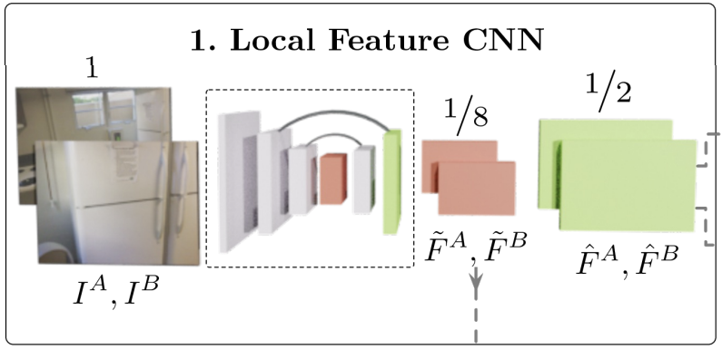
Architecture
Paper2: LoFTR
Architecture Abstract
Transformer를 기반으로 Pixel-wise Dense Match를
목표로 하는 모델
Procedure
ⅰ. Local Feature CNN
$\quad$ ◆ CNN을 거쳐 이미지로부터 Low Level Feature를
$\quad\;\,$ 추출한다.
$\quad \; \, \rightarrow$($\frac{1}{8}H, \frac{1}{8}W$)의 크기
$\quad$ ◆ UNet구조와 비슷하게 Low Level Feature를
$\quad \;\,$ Upsampling하여 더 정교한 Feature를 추출한다.
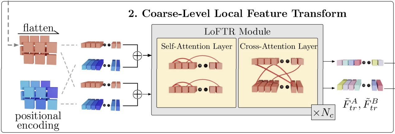
$\quad \; \, \rightarrow$ ($\frac{1}{2}H, \frac{1}{2}W$)의 크기
ⅱ. Coarse-Level Local Feature Transform
$\quad$ ◆ Flatten + Positional Encoding
$\quad \;\, \rightarrow$ DeTR과 비슷한 방식으로 Transfomer의 입력을
$\qquad \;$ 위한 준비과정
$\quad$ ◆ LoFTR Module
$\quad\;\, \rightarrow$ Self Attention으로 Patch내의 주요 특징 추출
$\quad\;\, \rightarrow$ Cross Attention으로 Image Matching Pair 생성

$\therefore$ ($\frac{1}{2}H, \frac{1}{2}W$)의 Coarse한 Feature로부터
$\quad$ Feature Vector를 구함
$\,$
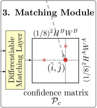
ⅲ. Matching Module
$\quad$ ◆ Differentiable Matching Layer
$\quad\;\, \rightarrow$ 두 Feature Vector의 유사도를 계산하여
$\qquad \;$ Confidence Matrix를 만듦
$\quad$ ◆ Confidence Matrix
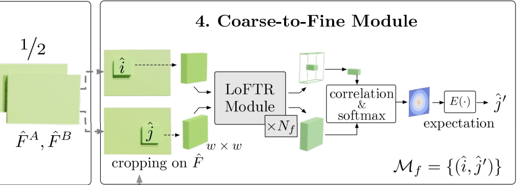
$\quad\;\, \rightarrow$ i가 J와 Matching될 확률(대칭행렬은 아님)
ⅳ. Coarse-to-Fine Module
$\quad$ ◆ Crop
$\quad\;\, \rightarrow$ 처음에 얻은 ($\frac{1}{2}H, \frac{1}{2}W$)의 두 Feature Map에서
$\qquad\;$ i, j Pixel을 중심으로한 Patch를 Crop
$\quad$ ◆ LoFTR Module
$\quad\;\, \rightarrow$ 두 Patch간의 유사도 검증
※ Coarse: 조잡한(정제되지 않은?)
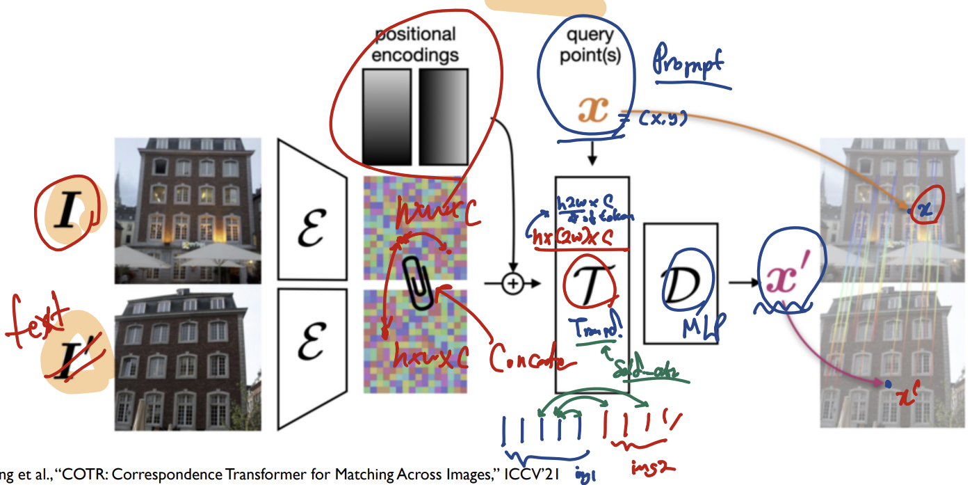
Paper3: COTR
중간에 Concatenate하고 Self Attention을 해줌으로써 Cross Attention(Image Matching)의 효과를 얻을 수 있음
Matching Point인 x’을 찾기위해 x를 Query로 사용

Architecture	Abstract
	Transformer를 기반으로 Pixel-wise Dense Match를 목표로 하는 모델

Procedure
	ⅰ. Local Feature CNN $\quad$ ◆ CNN을 거쳐 이미지로부터 Low Level Feature를 $\quad\;\,$ 추출한다. $\quad \; \, \rightarrow$($\frac{1}{8}H, \frac{1}{8}W$)의 크기 $\quad$ ◆ UNet구조와 비슷하게 Low Level Feature를 $\quad \;\,$ Upsampling하여 더 정교한 Feature를 추출한다. $\quad \; \, \rightarrow$ ($\frac{1}{2}H, \frac{1}{2}W$)의 크기
	ⅱ. Coarse-Level Local Feature Transform $\quad$ ◆ Flatten + Positional Encoding $\quad \;\, \rightarrow$ DeTR과 비슷한 방식으로 Transfomer의 입력을 $\qquad \;$ 위한 준비과정 $\quad$ ◆ LoFTR Module $\quad\;\, \rightarrow$ Self Attention으로 Patch내의 주요 특징 추출 $\quad\;\, \rightarrow$ Cross Attention으로 Image Matching Pair 생성 $\therefore$ ($\frac{1}{2}H, \frac{1}{2}W$)의 Coarse한 Feature로부터 $\quad$ Feature Vector를 구함 $\,$
	ⅲ. Matching Module $\quad$ ◆ Differentiable Matching Layer $\quad\;\, \rightarrow$ 두 Feature Vector의 유사도를 계산하여 $\qquad \;$ Confidence Matrix를 만듦 $\quad$ ◆ Confidence Matrix $\quad\;\, \rightarrow$ i가 J와 Matching될 확률(대칭행렬은 아님)
	ⅳ. Coarse-to-Fine Module $\quad$ ◆ Crop $\quad\;\, \rightarrow$ 처음에 얻은 ($\frac{1}{2}H, \frac{1}{2}W$)의 두 Feature Map에서 $\qquad\;$ i, j Pixel을 중심으로한 Patch를 Crop $\quad$ ◆ LoFTR Module $\quad\;\, \rightarrow$ 두 Patch간의 유사도 검증

Artificial Intelligence, Computer Vision

visual correspondence vision

	Image에서 Keypoint별로 $4 \times 4$개의 Window로 나눈다. 그리고 이 Window를 다시 $4 \times 4$개의 Sub-Window에 할당한다. (총 $16 \times 16$으로 나뉨) 마지막으로 각 구역별로 Image Pixel값에 기반해 Gradient를 계산한다.
	이 Gradient들을 Noise에 Robust하게 작동하도록 하기 위해 Gaussian Filter를 적용해준다.
	이제 Window별로 할당된 모든 구역에 대해 8개의 방향을 갖는 Orientation Histogram을 그린다. (Window당 $8 \times 4 \times 4 = 128$차원의 Vector가 생긴다.)
	완성