2. Search

Background

1) Define

인공지능이 문제를 해결할 때 사용할 수 있는 방법은 앞으로 취할 수 있는 행동들을 미리 시뮬레이션 해보고, 최적의 결과를 내는 행동을 찾는 것이다.

이때, Uninformed Search는 이 최적의 결과가 무엇인지 알 수 없는, 즉 목표까지 얼마나 남았는지 알 수 없는 상태(Uninformed)에서 행동을 찾는 알고리즘이다.

반면에 Informed Search는 이 목표가 정해져 있는 상황에서 행동을 찾는 알고리즘이다.

2) Terms

State

• 인공지능이 행동을 했을 때, 가능한 상태를 의미한다. 필요없는 Detail들을 제거하는 추상화, 간략화 과정이 필요하다.
  (ex. 바둑을 둘 때, 내가 돌을 두고 난 상태)
  • Initial State: 초기 상태
  • State Space: State들로 이루어진 집합
  • Search Tree: State Space를 방향 Graph가 아닌 Tree로 표현하는 것
  • Graph Search: State를 방향 Graph로 표현해 Solution을 찾는 것

(visited를 조사 O: Graph Search)
(visited를 조사 X: Tree Search)

(tree like: memory $\downarrow$)
(graph: memory $\uparrow$)

---

Action

• 현재 State에서 내가 취할 수 있는 모든 행동들을 의미한다.
  (ex. 바둑판에 바둑돌이 없는 칸에 돌을 두는 것)
  • Path: Action들로 이루어진 집합
  • Solution: Path들 중 목표까지 갈 수 있는 Path

---

Performance Evaluation

Completeness	Cost Optimality	Time Complexity	Space Complexity
1. Solution을 반드시 찾는지 2. Solution이 없다면 알 수 있는지	최적의 Solution을 찾는지	시간 복잡도	공간복잡도

1. Uninformed Search

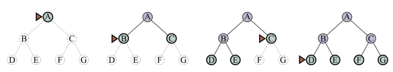
1) BFS

	평가함수$f(n)$	Completeness	Cost Optimal	시간복잡도	공간복잡도
BFS	Action 수	O	X	$O(b^d)$	$O(b^d)$
Dijkstra	Start Node $\overset{Cost}{\leftrightarrow}$ Current Node	O	O	$O(b^{1+\frac{C^*}{\epsilon}})$	$O(b^{1+\frac{C^*}{\epsilon}})$

$b$: Branch factor
$d$: solution의 depth
$\epsilon$: action의 최소 Cost
$C^*$: Optimal Solution의 Cost

FIFO(Firt In First Out)을 기반으로 구현하는 알고리즘이다.

def bfs(graph, start, end):
  frontier = queue([start])
  visited = [start]
  while not frontier.is_empty():
      node = frontier.pop()
      for child in expand(node, graph):
          if child.state == end:
              return child
          elif child not in visited:
              visited.append(child)
              frontier.append(child)
  return False

---

Uniform-Cost Search (Dijkstra)

def dijkstra(graph, start, end)
  frontier = heapq([start]).set(node.cost)
  visited = [start]
  while not frontier.is_empty:
      node = frontier.pop()
      if node.state == end:
          return node
      for child in expand(node, graph):
          if (child not in visited) or (child.cost < visited.find(child).cost):
              visited[visited.find(child)] = child
              frontier.append(child)
  return False

BFS에서 Heap과 같은 Priority Queue를 사용하고
Goal test는 원래의 BFS보다 나중에 해서 Cost Optimal을 보장해 준다.
(단, Cost는 0보다 커야함)

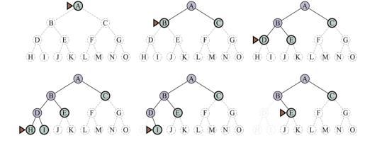
2) DFS

	Completeness	Cost Optimality	Time Complexity	Space Complexity
DFS	O(finite state space) X(infinite state space)	X	$O(b^m)$	$O(b^m)$(graph like) $O(bm)$(tree like)
BackTracking	O(finite state space) X(infinite state space)	X	$O(b^m)$	$O(m)$
Depth-Limited	X	X	$O(b^l)$	$O(bl)$
Iter-Deepening	O	X	$O(b^d)$	$O(bd)$

$b$: Branch factor
$d$: Solution의 depth
$m$: Maximum depth
$l$: Depth Limit

LIFO(Last In First Out)을 기반으로 구현하는 알고리즘이다.

---

Back Tracking

DFS는 Node의 모든 Child를 바로 생성하여 각 Child의 조건을 검사한다.

하지만 Back Tracking은 메모리를 아끼기 위해 한번에 하나씩 생성하여 조건을 검사해간다.

---

Depth-Limited Search

일반적인 DFS는 무한 roop에 빠질 수 있다.
이를 막기위해 ⅰ. Cycle을 확인하고, 뻗을 수 있는 Depth에 ⅱ. Limit을 설정하여 그 이상은 Cutoff한다.

def DLS(graph, start, end, limit):
  frontier = stack([start])
  cutoff = False
  while not frontier.is_empty():
      node = frontier.pop()
      if node.state == end:
          return node
      if node.depth > limit:
          cutoff = True
      elif not cycle(node):
          for child in expand(node, graph):
              frontier.append(child)
  return cutoff

---

Iterative Deepening Search

Depth Limit을 0부터 $\infty$까지 증가해가며 Depth Limited Search를 진행하는 방식

---

Iterative Lengthning Search

Cost Limit를 0부터 $\infty$까지 증가시키며 Search하는 방식

이때, 다음 Cost는 연속적이기 때문에 다음 Iter의 Limit은 이전 Iter의 최솟값으로 한다.

---

Hybrid Approach

DFS는 시간이 오래걸린다.
따라서 BFS로 메모리가 어느정도 찰 때 까지는 탐색하다가 Iterative Deepening으로 바꾸는 전략을 쓸 수도 있다.

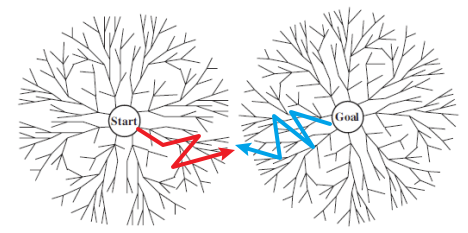
3) Bidrectional Search

	Completeness	Cost Optimality	Time Complexity	Space Complexity
Bidirectinal	O	X	$O(b^\frac{d}{2})$	$O(b^\frac{d}{2})$

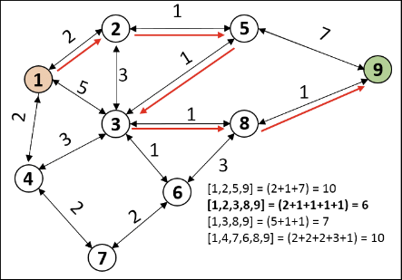
Goal State를 알 때 쓸 수 있는 방법으로 Goal지점과 Start지점에서 모두 Dijkstra 방법으로 Search를 시작하는 방법이다.

def bid(graph_f, front, graph_b, back):
  frontier_f = heapq([front]).set(node.cost)
  frontier_b = heapq([back]).set(node.cost)

  visited_f = [front]
  visited_b = [back]

  solution = False

  while not Terminated:
      if frontier_f.top().cost < frontier_b.top().cost:
          solution = proceed(graph_f, frontier_f, visited_f, visited_b)
      else:
          solution = proceed(graph_b, frontier_b, visited_b, visited_f)

def proceed(graph, cost, frontier, visited_1, visited_2, solution):
  node = frontier.pop()
  for child in expand(node, graph):
      if (child not in visited_1) or child.cost < visited_1.find(child).cost:
          visited[visited_1.find(child)] = child
          frontier.append(child)
          if child in visited_2:
              solution_temp = join(child, visited_2[child])
              if solution_temp.cost < solution.cost:
                  solution = solution_temp
  return solution

(이때, 먼저 연결되었다고 해서 Cost Optimal이라는 보장이 없다.)

---

2. Informed(Heuristic) Search

1) Best-First Search

	평가함수$f(n)$	Completeness	Cost Optimal	시간복잡도	공간복잡도
GBFS	Current Node $\overset{Cost}{\leftrightarrow}$ Goal Node	X(graph like) O(tree like)	X	$O(b^m)$	$O(b^m)$
$A^*$	Start Node $\overset{Cost}{\leftrightarrow}$ Current Node $+$ Current Node $\overset{Cost}{\leftrightarrow}$ Goal Node	O	O	$x \leq O(b^d)$	$x \leq O(b^d)$
$SMA^*$		O	O	$x \leq O(b^d)$	$x \leq O(b^d)$

각 Node들에 대해 평가함수 $f(n)$이 가장 작은 Node들을 확장해 나가며 Search하는 알고리즘이다.
따라서 주로 HEAP을 기반으로 구현한다.

def Best_First_Search(graph, start, end, cost_func):
  frontier = heapq([start]).set(cost_func(node))
  visited = [start]
  while not frontier.is_empty():
      node = frontier.pop()
      if node.state == end:
          return node
      for child in expand(node, graph):
          if (child not in visited) or (cost_func(child) < cost_func(visited.find(child))):
              visited[visited.find(child)] = child
              frontier.append(child)
  return False

이때 $f(n)$으로 휴리스틱 함수를 사용하기도 하는데 다음에 주의하자

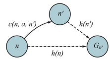
※ $H(n)$

Optimal Heuristic Function	Consistent Heuristic Function
$h(n) \leq h^*(n)$	$h(n) \leq c(n, n_{next}) + h(n_{next})$
실제 거리보다 예측 거리가 항상 클 때 Optimal하다.	즉, 다음 Node에서의 Goal까지의 거리가 현재 Node에서 Goal까지의 거리보다 항상 작을 때 (Optimal보다 더 까다로운 조건이다.)

---

Greedy Best-First Search

def Greedy_Best_First_Search(graph, start, end, cost_func):
  def cost_func(node):
      return distance(node, end)
  return Best_First_Search(graph, start, end, cost_func)

평가함수가 현재노드부터 Goal Node까지의 Heuristic 추정 거리이다.

---

$A^*$ Search

def A_star(graph, start, end, cost_func):
  def cost_func(node):
      return node.cost + distance(node, end)
  return Best_First_Search(graph, start, end, cost_func)

평가함수가 시작Node부터 현재Node까지의 실제 거리와 현재Node부터 Goal Node까지의 추정 거리를 합한 함수이다.

---

Iterative Deepening $A^*$ Search

iterative Deepening(Lengthning) Search와 비슷하게 limit cost를 정한 후 이를 반복적으로 갱신하며 $A^*$ Search를 수행하는 알고리즘이다.

마찬가지로 반복시 cost는 이전 cost의 최솟값으로 갱신한다.

---

Simpleified Memory-Bounded $A^* $ Search ($SMA^*$)

$A^*$를 메모리가 가득 찰때까지 수행하다가
메모리가 가득차면 가장 높은 Cost를 갖는 node들부터 drop해가며 계산하는 방식

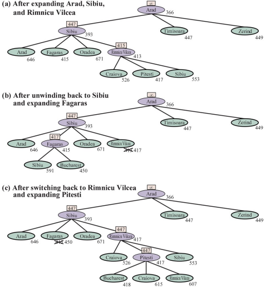
2) Recursive Best-First Search (RBFS)

	Completeness	Cost Optimality	Time Complexity	Space Complexity
RBFS	O	O	$O(b^d)$	$O(bd)$

Depth First와 $A^*$를 결합한 방식

def RBFS(graph, start):
  solution, f = _RBFS(graph, start, 1e9)
def _RBFS(graph, node, f_limit):
  children = expand(node, graph)
  if children.is_empty:
      return False, 1e9
  for child in children:
      child.f = max(child.cost + h(child), node.f)
  while True:
      child.sort()
      best, alternative = child[0], child[1]
      if best.f > f_limit:
          return False, best.f
      result, best.f = _RBFS(graph, best, f_limit = min(f_limit, alternative.f))
      if result != False:
          return result, best.f

	1. Sibling 생성
	2. best($f(n)$이 가장 낮은 것)와 　alternative(두번째로 낮은 것) 설정
	3. 만약 $best.f$가 f_limit보다 　커지면 best.f를 return
	4. parent와 alternative의 f_limit 중 　작은 값을 사용해 다시 RBFS 반복
	5. 현재 Node(best)의 f값은 　return될 RBFS의 f값으로 설정