6. Object Detection(One-Stage)

Object Detection

1. One-Stage Detection Model

1) YOLO

Purpose

1. 앞선 모델들은 ROI를 위해 Box Regression과정을 한번 더 수행했다.
   $\rightarrow$ Grid Cell

(논문 제목 그대로 You Only Look Once, Box Regression과정은 한번이면 족하다.) (제목부터 자극적이다…)

---

동작과정

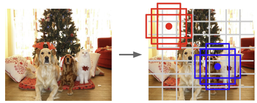
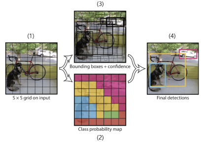
1. Grid

   이미지를 $7 \times 7$크기의 Grid로 나눈다.
   

2. Classification
   

   각 Grid에 대해 Classification을 수행한다.
   (Background도 이 Class중 1개에 포함)

3. Base Box 생성
   

   각 Grid에 대해 “B”개의 Base Box들을 생성한다.
   (이 Base Box가 Anchor Box의 역할을 함)

4. 각 Base Box별로 Regression을 수행한다.
   Output $\rightarrow$ (x, y, h, w, Confidence)
   (grid cell기준 x, grid cell기준 y, image기준 h, image기준 w, objectness)

$\therefore 7 \times 7\times (5 \times B + C)$개의 Bounding Box 생성

2) DETR

Purpose

1. 기존의 Anchor Box를 사용하는 방식은 다음과 같다.
   Positive Sample 결정 $\rightarrow$ NMS (or other Hand Craft Post Processing) $\rightarrow$ ROI결정
   즉, Ground Truth에 대해 Prediction이 Many-to-one 관계이다.
   
   $\Rightarrow$ Anchor Box을 없애 Hand craft한 Post Processing이 없는 One-to-one model을 만듦

---

동작과정

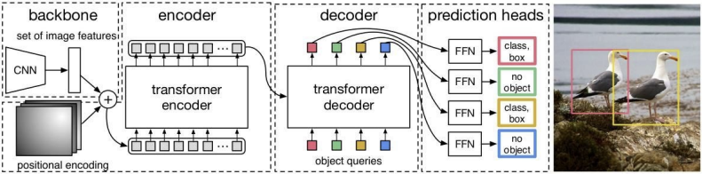
과정
1. Backbone		$(C, H, W)$ $\rightarrow (D, HW)$	ⅰ. Flatten 　: Transformer의 Query로 주기 위한 평탄화 ⅱ. Positional Encoding 　: Patch의 위치정보를 위한 Encoding
2. Transformer (Encoder)		$(D, HW)$ $\rightarrow (D, HW)$	Encoder는 Multi-head Self Attention을 통해 Key와 Value를 생성
3. Transformer (Decoder)		$(D, HW), N$ $\rightarrow N$	ⅰ. N개의 Object Query(초기값=0) 생성하고 　Multi-head Self Attention ⅱ. Encoder의 Key-Value와 함께 　Multi-head Cross Attention ☆ Query는 Object Prompt & Learnable
4. Feed Foward		$N \rightarrow N$	ⅰ. N개의 Query에 대해 모두 예측 　(Background의 경우 예측 X) ⅱ. Set to Set 학습을 위한 　Bipartite Matching

(Self Attention: Query, Key, Value가 같은 Feature Map에서 생성되는 것)
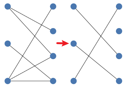
(Cross Attention: Query는 생성 Key, Value를 Encoder에서 가져오는 것)

---

Bipartite Matching

DETR은 Output이 Parallel하게 출력된다. 즉, Box Regression결과를 한번에 알게 된다.

따라서 각 Box가 어떤 Ground Truth와 Matching되어야 하는지 알 수 없다.

이때, Brute Force하게 최적의 조건을 탐색하면 시간이 지나치게 많이 걸린다.
이를 위해 사용하는 것이 Bipartite Matching(이분 매칭)으로, 각 Bounding Box가 어떤 Ground Truth와 연결되어야 최적의 상태가 되는지 알아내는 알고리즘이다.

\[\hat{\sigma} = \text{arg}\,\min \limits_{\sigma \in \Omega_N} \sum \limits_i^N \mathcal{L}_{match}(y_i, \hat{y}_{\sigma(i)})\]

• 최적의 쌍($\hat{\sigma}$)은 두 노드를 잇는 연결선 중($\sigma \in \Omega_N$) 유사도($\mathcal{L}_{match}$)를 최소화 하는 쌍

\[\mathcal{L}_{match} = -\mathbb{1}_{\{c_i \neq \emptyset\}} \hat{p}_{\sigma(i)}(c_i) + \mathbb{1}_{\{c_i \neq \emptyset\}} \mathcal{L}_{box}(b_i, \hat{b}_{\sigma(i)})\]

　 \(\mathcal{L}_{Hungarian}(y, \hat{y}) = \sum \limits_{i=1}^N [-log(\hat{p}_{\hat{\sigma}(i)}(c_i)) + \mathbb{1}_{\{c_i \neq \emptyset\}} \mathcal{L}_{box}(b_i, \hat{b}_{\hat{\sigma}}(i))]\)

　

– todo: SSD, RetinaNet, Efficient Det, M2Det, CorNerNet –