5. Algorithm
1. Unconstrained Minimization
\[\text{Minimize: } f(\mathbf{x})\]$\mathbf{x} \in \mathbb{R}^n,$
$f(\mathbf{x}) \text{는 Convex},$
$f(\mathbf{x}) \text{는 두번 미분 가능}$
Background
Minimization을 Algorithm으로 구현할 때의 핵심은 $f(x^{(n)}) = p^*$일 때, Iterative Method를 사용해 KKT Condition을 만족할 때 까지 $x^{(0)}, x^{(1)}, … , x^{(n)}$점으로 진행하는 것이다.
이때, Unconstrained문제이므로 이 최적점 $\mathbf{x}^{(n)}$는 결국 $\nabla f(\mathbf{x}^*) \approx 0$을 만족할 것이다.
이 점을 찾기 위해서 Descent Method를 사용할 수 있는데, 이 방법의 핵심은 다음과 같다.
\[\mathbf{x}^{(k+1)} = \mathbf{x}^{(k)} + t^{(k)} \vartriangle \mathbf{x}^{(k)} \\ f(\mathbf{x}^{(k)}) > f(\mathbf{x}^{(k+1)})\]
먼저 Convex함수이기 때문에 항상 내려가는 방향으로 움직이기만 하면 된다.$\vartriangle \mathbf{x}$는 방향
$t > 0$는 크기즉, 위 식을 만족하는 $f(\mathbf{x}^{(k+1)})$을 찾아야 하는데, 이를 찾기 위해 다음의 사실을 이용할 수 있다.
$f(\mathbf{x}^{(k+1)}) > f(\mathbf{x}^{(k)}) + \nabla f(\mathbf{x}^k)(\mathbf{x}^{k+1} - \mathbf{x}^k) \rightarrow$ (Convex의 정의)즉, 해당 지점에서의 미분값과 크기를 $\nabla f(\mathbf{x}^{(k)})^T \vartriangle \mathbf{x}^{(k)} < 0$를 만족하도록 정의하면 된다.
Line Search
이제 이동할 크기(Learning Rate)를 정하는 방법을 먼저 살펴보자
Exact Line Search Backtracking Line Search $t = \text{arg} \min \limits_{t > 0} f(\mathbf{x} + t \vartriangle \mathbf{x})$ $f(\mathbf{x} + t \vartriangle \mathbf{x}) < f(\mathbf{x}) + \alpha t \nabla f(\mathbf{x})^T \vartriangle \mathbf{x}$ t만큼 움직였을 때, 함수값이 가장 작아질 때 현재위치에서 접선의 기울기보다
기울기의 절댓값을 줄인 직선보다
아래에 있을 때t에 대해 Restriction to a line이기 때문에
Convex함수 이므로 Minimization문제를 푼다
ⅰ. $t=1, \alpha \in (0, \frac{1}{2}), \beta \in (0, 1)$로 Setting
ⅱ. $t = \beta t$를 위 식을 만족할 때 까지 반복단점
: Convex문제를 풀어야하기 때문에 복잡도 $\Uparrow$생각보다 성능이 좋다.
위에서는 learning rate들을 정할 수 있는 몇가지 방법을 알아보았으니 이제 방향 등 자세한 방식들을 알아보자.
1) Gradient Descent
$\mathbf{x}$에서 움직일 방향을 Gradient로 설정하는 방식이다.
\[\mathbf{x}^{(k+1)} = \mathbf{x}^{(k)} + t^{(k)} \vartriangle \mathbf{x}^{(k)}\]| Gradient Descent | Steepest Descent | |
|---|---|---|
| $\vartriangle x$ | $\vartriangle x = -\nabla f(\mathbf{x})$ | ⅰ. Normalized $\quad \vartriangle x_{nsd} = \text{arg}\min \limits_{\Vert v \Vert_P \leq 1} (\nabla f(\mathbf{x})^T v)$ $\quad$(Gradient Descent의 일반화 ver) $\quad$(v에 대한 Norm) ⅱ. Unnormalized \(\quad \vartriangle x_{sd} = \Vert \nabla f(\mathbf{x}) \Vert_* \vartriangle \mathbf{x}_{nsd}\) $\,$ |
| 목표 | 현재 기울기가 가장 가파른 곳으로 이동 Unnormalized Steepest Descent의 2-norm ver | $f(\mathbf{x} + v) \approx f(\mathbf{x}) + \nabla f(\mathbf{x})^Tv$ $v$만큼 움직였을 때 함숫값이 최소가 되도록 $\,$ |
| 해법 | 현재 위치에서 Jacobian을 구한다. | \(\text{Minimize} \qquad \nabla f(\mathbf{x})^T v \\ \text{Subject to} \qquad \Vert v \Vert_P \leq 1\) 문제 이므로 Convex Optimization 문제 |
| L1-Norm | Euclidean Norm | Quadratic Norm | |
|---|---|---|---|
| $\vartriangle \mathbf{x}_{nsd}$ | \(-\frac{\nabla f(\mathbf{x})}{\Vert \nabla f(\mathbf{x}) \Vert_2}\) | ||
| $\vartriangle \mathbf{x}_{sd}$ | \(\Vert \nabla f(\mathbf{x}) \Vert_2 \times -\frac{\nabla f(\mathbf{x})}{\Vert \nabla f(\mathbf{x}) \Vert_2}\) \(\therefore - \nabla f(\mathbf{x})\) | \(\therefore -P^{-1}\nabla f(\mathbf{x})\) |
Convergence rate
$f(\mathbf{x})$가 Strongly Convex일 경우 다음 식을 항상 만족한다.
\[f(\mathbf{x}^{(k)}) - p^* \leq c^k (f(\mathbf{x}^{(0)}) - p^*)\]즉, Convergence가 보장된다.
(c가 작을수록 Convergence 속도는 느려짐)※ Strongly Convex: $\nabla f(\mathbf{x}) - mI\succeq 0$
$\quad$(휘어짐의 정도(곡률)이 $mI$보다 큼)Algorithm
단점
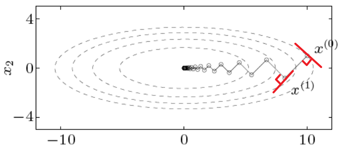
수렴 속도 P의 설정 Gradient Descent는 현재 위치에서의 기울기,
즉 Local한 정보만을 활용하기 때문에
수렴 속도가 매우 느리다.P의 설정에 따라 수렴 속도가 매우 달라짐
예시 그림 \(f(\mathbf{x}) = \mathbf{x}_1^{2} + \gamma \mathbf{x}_2^2, \gamma > 0\)
\(\mathbf{x}^{(0)} = (\gamma, 1) \quad \text{& Exact Line Search}\)
\(\therefore \mathbf{x}_1^{(k)} = \gamma(\frac{\gamma - 1}{\gamma + 1})^k, \quad \mathbf{x}_2^{(k)} = (-\frac{\gamma - 1}{\gamma + 1})^k\)$\qquad \Rightarrow$ Oscillate 발생
2) Newton’s Method
| Interpretation | 그림 |
|---|---|
| ⅰ Local Hessian Norm $\quad$ Gradient Descent는 Local한 정보($\nabla f(\mathbf{x})$)만 $\quad$ 이용했기 때문에 문제가 발생하였다. $\quad$ 즉, Global한 정보인 Hessian을 고려해야 하고 $\quad$ 이를 위해 방향마다 거리를 다르게 설정하는 $\quad$ Quadratic Norm을 활용할 수 있다. \(\quad \therefore P = \nabla^2 f(\mathbf{x})\) \(\quad \rightarrow \vartriangle \mathbf{x}_{sd} = - (\nabla^2 f(\mathbf{x}))^{-1}(\nabla f(\mathbf{x}))\) ⅱ. Taylor Series $\quad f(\mathbf{x})$를 $\mathbf{v}$만큼 움직였을 때의 함수를 $\quad$ Taylor Series의 2차항까지로 표현하면 $\quad$ 다음과 같다. \(\quad f(\mathbf{x + v}) \approx f(\mathbf{x}) + \nabla f(\mathbf{x})\mathbf{v} + \frac{1}{2} \mathbf{v}^T \nabla^2 f(\mathbf{x})\mathbf{v}\) $\quad$ 즉, 이 2차함수를 최소화하는 $\mathbf{v}$를 찾으면, $\quad \mathbf{v} = \vartriangle \mathbf{x} = -\frac{\nabla f(\mathbf{x})}{\nabla^2 f(\mathbf{x})}$이다. | 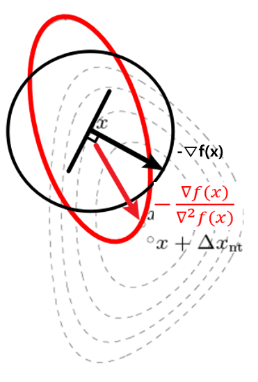 |
Newton’s Method는 위의 두가지 관점으로 해석할 수 있다.
Newton Decrement (Stopping Criterion)
Newton Decrement는 다음과 같이 정의된다.
\[\lambda(\mathbf{x}) = (\nabla f(\mathbf{x})^T \nabla^2f(\mathbf{x}^{-1}) \nabla f(\mathbf{x}))^{\frac{1}{2}} \\ \quad = (\vartriangle \mathbf{x}_{nt}^T \nabla^2 f(\mathbf{x}) \vartriangle \mathbf{x}_{nt})^\frac{1}{2}\]이때, Newton Decrement는 다음과 같은 특징을 갖는다.
$f(\mathbf{x}) - \inf \limits_y \hat{f}(y) = \frac{1}{2} \lambda(\mathbf{x})^2$즉 이 Newton Decrement가 0 에 가깝다면 최적점에 가까워졌다고 할 수 있고
따라서 이를 Stopping Criterion으로 사용할 수 있다.Algorithm
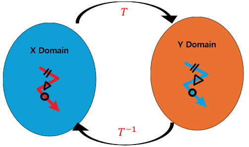
특징
- $\mathbf{x}$에 대한 함수를 $\mathbf{y} = T^{-1}\mathbf{x}$에 대한 함수로 Transform하더라도 Newton’s Method를 사용해 이동할 경우 Mapping관계가 그대로 유지된다.
2. Constrained Minimization
1) Equality Constrained Optimization
| Problem | KKT Condition |
|---|---|
| \(\text{Minimize: } \quad f(\mathbf{x}) \\ \text{Subject to}: \quad A\mathbf{x} = \mathbf{b}\) $A \in \mathbb{R}^{p \times n},$ $Rank(A) = p$ $\mathbf{x} \in \mathbb{R}^n,$ $f(\mathbf{x}) \text{는 Convex},$ $f(\mathbf{x}) \text{는 두번 미분 가능}$ | \(\text{Primal Feasible: } \; \qquad A\mathbf{x}^* = \mathbf{b}\) \(\text{Gradient of Lagrangian: } \quad \nabla f(\mathbf{x}^*) + A^T\nu^* = 0\) ※ Dual Residual: $r_d(\mathbf{X}, \nu) = \nabla f(\mathbf{x}) + A^T\nu$ ※ Primal Residual: $r_p(\mathbf{x}, \nu) = A\mathbf{x} - \mathbf{b}$ |
※ Equality Constrained Quadratic Minimization일 경우 주의할 점이 필요하므로 이를 살펴보자.
| Problem | KKT Matrix |
|---|---|
| \(\text{Minimize: } \quad \frac{1}{2} \mathbf{x}^{*T}P\mathbf{x}^* + q^T\mathbf{x}^* + r\) \(\text{Subject to}: \; A\mathbf{x} = \mathbf{b}\) —————————————————– KKT Condition \(P\mathbf{x}^* + q + A^T \nu = 0\) \(A\mathbf{x}^* = \mathbf{b}\) \(\qquad \Downarrow\) \(\begin{bmatrix} P & A^T \\ A & 0 \end{bmatrix} \begin{bmatrix} \mathbf{x}^* \\ \mathbf{\nu}^* \end{bmatrix} = \begin{bmatrix} -q \\ \mathbf{b} \end{bmatrix}\) | \(K = \begin{bmatrix} P & A^T \\ A & 0 \end{bmatrix}\) 이때 문제를 풀기위해 KKT Matrix가 Non-Singular Matrix(역함수 존재)임을 가정하자. $\Rightarrow \mathcal{N}(P) \cap \mathcal{N}(A) = \begin{Bmatrix} 0\end{Bmatrix}$ $\Rightarrow \mathbf{x}^TP\mathbf{x} + \Vert A\mathbf{x} \Vert^2 > 0 \quad \because$(P:정방행렬, A:비정방행렬) $\Rightarrow P + A^TA \succ 0$ 즉, 위 식이 성립하면 Unique한 Solution을 구할 수 있다. (또 만약 $P \succ 0$일 경우에도 마찬가지이다.) |
Eliminating Equality Constraint
KKT Condition으로도 문제를 풀 수는 있다.
하지만 앞서 배운 Unconstrained Optimization에서 사용하는 알고리즘들(Gradient Descent, Newton’s Method)를 사용하기 위해서는 Constraint를 없애줄 필요가 있다.
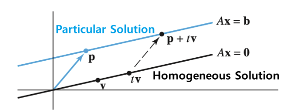
$\mathbf{x} = \mathbf{x}_h + \mathbf{x}_p$ Nonhomogeneous System에서 배웠듯이 $A\mathbf{x} = \mathbf{b}$의 해는
Homogeneous Solution($A\mathbf{x} = 0$)과
Particular Solution($A\mathbf{x} = \mathbf{b}$)으로 나눌 수 있다.이를 이용하여 Constraint가 존재하는 $\mathbf{x}$는 Constraint가 존재하지 않는 $\mathbf{z}$에 대한 식으로 바꿀 수 있다.
\(\qquad \begin{Bmatrix} \mathbf{x} \vert A \mathbf{x} = b \end{Bmatrix} \rightarrow \begin{Bmatrix} F\mathbf{z} + \hat{\mathbf{x}} \vert \mathbf{z} \in \mathbb{R}^{n-p} \end{Bmatrix} \\ \, \\F \in \mathbb{R}^{n \times (n-p)} \\ AF = 0, \quad (\mathcal{N}(A) = F)\\ A\mathbf{\hat{x}} = \mathbf{b} \qquad \qquad \qquad \quad\) \(\Rightarrow \qquad \underset{z}{\text{Minimize}} \quad f(F\mathbf{z} + \hat{x}) \qquad \qquad\) 즉 이 Unconstrained Minimization Problem의 해 $\mathbf{z}^*$를 구하고
$\mathbf{x}^* = F\mathbf{z}^* + \hat{\mathbf{x}}, \quad \nabla f(\mathbf{x}^*) + A^T \nu^* = 0$를 통해 원래의 해($\mathbf{x}^*, \nu^*$)를 알 수 있다.Projected Gradient Method
다음 3개의 문제를 살펴보자.
Problem1 Problem2 Problem3 \(\underset{\mathbf{x}}{\text{Minimize}} \quad f(\mathbf{x}) \\ \text{Subject to} \quad A\mathbf{x} = \mathbf{b}\) \(\underset{z}{\text{Minimize}} \quad f(F\mathbf{z} + \hat{x})\) \(\underset{\mathbf{y}}{\text{Minimize}} \quad \Vert F\mathbf{y} - (-g) \Vert_2\) — \(\mathbf{z}^* = F^T \cdot \nabla_\mathbf{x} f(F\mathbf{z} + \hat{\mathbf{x}}) \\ \vartriangle\mathbf{z} = -\mathbf{z}^*\) \(\mathbf{y}^* = -F^Tg\)
(if $F$ is Orthonormal basis)우선 1번과 2번이 같은 문제임은 앞에서 증명하였다.
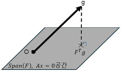
이때, 3번에서 $g= \nabla_\mathbf{z} f(F\mathbf{z} + \hat{\mathbf{x}})$라고 설정하면 2번문제의 Gradient Descent의 Step이 3번 문제의 Optimal인 점과 동일하다는 것을 알 수 있다.
즉, $g = \nabla_\mathbf{x} f$를 $F$가 Span하는 공간 위로 Projection시킨 벡터가 해임을 알 수 있다.
이를 통해 알 수 있는 것은 Equality Constrained일 경우,
Unconstrained일때의 Gradient Descent의 Step은 Equality Constrained일 때
$A$의 Null Space(즉, Homogeneous해) 평면 위로
Projection되어 진행한다는 것이다.Newton Step
Newton Step은 현재 위치에서 2차근사를 활용해 최솟값을 찾는 방식이다.
즉, 다음의 문제를 풀면된다.
Problem KKT Condition \(\underset{\mathbf{\nu}}{\text{Minimize:}}\; \hat{f}(\mathbf{x} + \mathbf{\nu}) = f(\mathbf{x}) + \nabla_\mathbf{x} f(\mathbf{x})^T \nu + \frac{1}{2} \nu^T \nabla^2_\mathbf{x} f(\mathbf{x}) \nu \\ \text{Subject to: }\quad A(\mathbf{x} + \nu) = \mathbf{b}\) ⅰ. Primal Feasible
\(A(\mathbf{x} + \nu) = \mathbf{b}\)
ⅳ. Gradient of Lagrangian
\(\nabla_\nu (\hat{f}(\mathbf{x} + \mathbf{\nu}) + A(\mathbf{x} + \nu) - \mathbf{b}) \\ = \nabla_\mathbf{x} f(\mathbf{x}) + \nabla^2_\mathbf{x}f(\mathbf{x}) \nu + A^Tw = 0\)즉 다음의 Linear Equation의 Solution이다.
\[\begin{bmatrix} \nabla^2_\mathbf{x} f(\mathbf{x}) & A^T \\ A & 0\end{bmatrix} \begin{bmatrix} \nu \\ W \end{bmatrix} = \begin{bmatrix} -\nabla_\mathbf{x} f(\mathbf{x}) \\ 0 \end{bmatrix}\]※ Newton Decrement: \(\lambda(\mathbf{x}) = (\vartriangle \mathbf{x}^T_{nt} \nabla^2 f(\mathbf{x}) \vartriangle \mathbf{x}_{nt})^\frac{1}{2} = (-\nabla f(\mathbf{x})^T \vartriangle \mathbf{x}_{nt})^\frac{1}{2}\)
2) Inequality Constrained Optimization
Irritation(Indicator) Function을 사용해서 Inequality로 바꾸자!
| Original Problem | Approximated Problem |
|---|---|
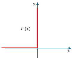 | 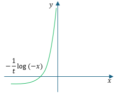 |
| \(\text{Minimize: } \quad f_0(\mathbf{x}) \\ \text{Subject to: } \quad f_i(\mathbf{x}) \leq 0 \\ \qquad\qquad \qquad A\mathbf{x} = \mathbf{b}\) $\qquad \qquad \Downarrow$ \(\text{Minimize: } \quad f_0(\mathbf{x}) + \sum \limits_{i=1}^m I_-(f_i(\mathbf{x})) \\ \text{Subject to: } \quad A\mathbf{x} = \mathbf{b}\) | \(\text{Minimize: } \quad f_0(\mathbf{x}) - \frac{1}{t} \sum \limits_{i=1}^m log(-f_i(\mathbf{x})) \\ \text{Subject to: } \quad A\mathbf{x} = \mathbf{b}\) ($t>0$는 Hyperparameter, 클수록 $I_-(x)$와 같아짐) (Log barrier function: $\phi (\mathbf{x}) = - \sum \limits_{i=1}^m log(-f_i(\mathbf{x}))$) |
$\nabla \phi(\mathbf{x}) = \sum \limits_{i=1}^m \frac{1}{-f_i(\mathbf{x})} \nabla f_i(\mathbf{x})$
$\nabla^2 \phi(\mathbf{x}) = \sum \limits_{i=1}^m \frac{1}{-f_i(\mathbf{x})^2} \nabla f_i(\mathbf{x}) \nabla f_i(\mathbf{x})^T + \sum \limits_{i=1}^m \frac{1}{-f_i(\mathbf{x})} \nabla^2 f_i(\mathbf{x})$
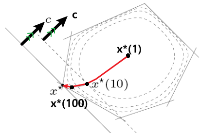
Central Path
\[\Downarrow\]
Approximated Problem에서 t를 곱하고
이 식의 t에 따른 Solution의 경로$\mathbf{x}^*(t)$를
Central Path라고 한다.
$\text{Minimize:} \quad tf_0(\mathbf{x}) + \phi(\mathbf{x})$
$\text{subject to:}\quad A\mathbf{x} = \mathbf{b}$
ex) $f_0(\mathbf{x}) = c^T\mathbf{x}$
$\quad f_i(\mathbf{x}) = a_i^T \leq b_i$$\text{KKT Condition(ⅰ): } A\mathbf{x} = \mathbf{b}$
\[\Downarrow\] \[f_0(\mathbf{x}^*(t) \geq p^* \geq g(\lambda^*(t), \nu^*(t))) \\ \qquad \qquad \qquad \qquad = L(\mathbf{x}^*(t), \lambda^*(t), \nu^*(t)) \\ \qquad \qquad \qquad \quad \qquad \qquad \qquad \quad = f_0(\mathbf{x}^*(t)) - \frac{m}{t} \quad (\text{m inequality #})\]
$\text{KKT Condition(ⅳ): } t \nabla f_0(\mathbf{x}) + \sum \limits_{i=1}^m \frac{1}{-f_i(\mathbf{x})} \nabla f_i(\mathbf{x}) + A^T \nu = 0$즉, 이 t의 크기를 통해 Optimal Value와의 오차를 조절할 수 있다.
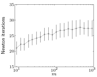
따라서, Stopping Criterion을 정하고 t를 점차 키워가면서 Optimal Value를 구하는 알고리즘을 사용할 수 있다.Algorithm
(t마다 Initial_x의 값을 계속 변화시키면서 Optimal을 찾는다.)
(전통적으로는 $\mu = 10 \sim 20$으로 설정한다.)
($\mu$가 너무 클 경우 Step을 계산하는 시간이 너무 오래걸린다. 즉, Trade off가 있다.)\[(\text{Central Path Complexity, via }\mu)\]